Here we provide information and data required to replicate the benchmark setup and evaluation protocol.

Abstract

We propose a new benchmarking protocol to evaluate algorithms for bimanual robotic manipulation semi-deformable objects. The benchmark is inspired from two real-world applications: (a) watchmaking craftsmanship, and (b) belt assembly in automobile engines. We provide two setups that try to highlight the following challenges: (a) manipulating objects via a tool, (b) placing irregularly shaped objects in the correct groove, (c) handling semi-deformable objects, and (d) bimanual coordination. We provide CAD drawings of the task pieces that can be easily 3D printed to ensure ease of reproduction ,and detailed description of tasks and protocol for successful reproduction, as well as meaningful metrics for comparison. We propose four categories of submission in an attempt to make the benchmark accessible to a wide range of related fields spanning from adaptive control, motion planning to learning the tasks through trial-and-error learning.

Authors: Konstantinos Chatzilygeroudis, Bernardo Fichera, Ilaria Lauzana, Fanjun Bu, Kunpeng Yao, Farshad Khadivar, and Aude Billard

Tasks

Benchmark Documents

Benchmark document: Benchmark

Protocol document (watchmaking task): Watch-making task

Protocol document (rubber-band task): Rubber-band task

Watchmaking Task

This task consists in completing one step of the assembly of a typical watch, namely inserting the plate, using a dual-arm robot system holding the required tools at their end-effector. This task poses the following main challenges to robotic systems:

• Manipulating objects via a tool;
• Placing an irregularly shaped object (the plate) in the correct groove that requires millimeter accuracy control;
• Handling a semi-deformable object: the plate’s leg;
• Multi-arm coordination: one arm stabilizing the system,and the other(s) performing the leg’s bending and final plate insertion.

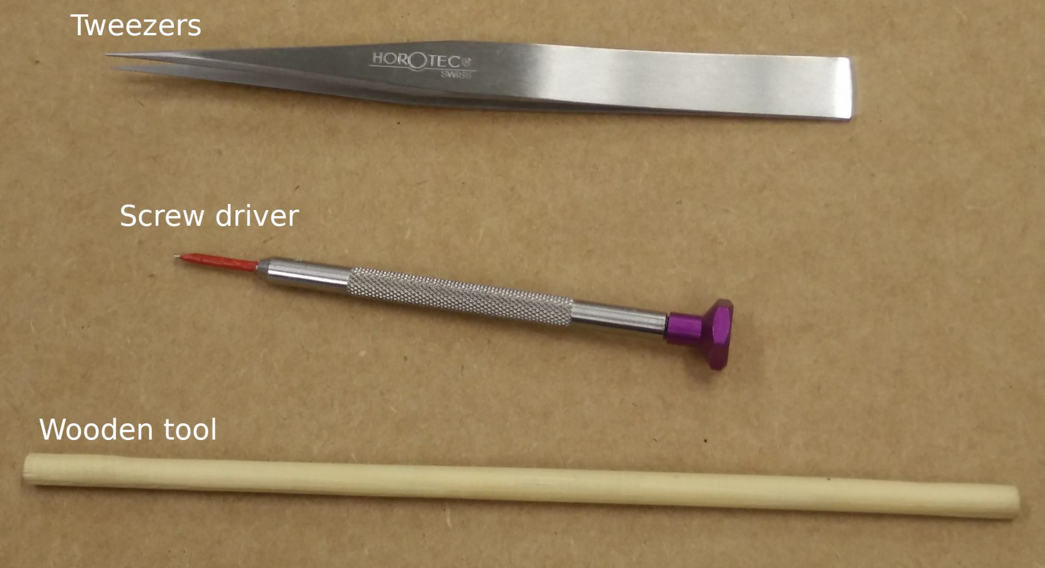
The plate is semi-deformable, and it necessitates bending in order to put it in place. Additionally, its small size requires the usage of a second tool to keep the object stable. The tools that are used in the actual setup are (shown in the following figure): the tweezers, a screwdriver and a wooden tool.

The task should be performed by a pair of robotic arms as follows (see figure below):

One arm holds/supports the tweezers at its end-effector,while the other arm holds/supports the stick (or similar tool)at its end-effector. At onset, the plate is already held stiffly in the tweezers (i.e., the robot does not have to pick it up).The arms must insert the plate in the correct location/groove on the watch face. This requires orienting the piece correctly and then bending its leg to stay in place.

Watch Pieces

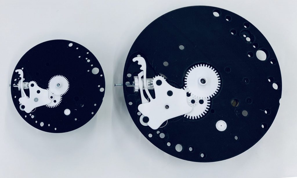
The real watch from which this task is inspired is quite small with a diameter of 37mm.

While, in the long run, many commercial solutions will be offered to robotic arms precise enough to manipulate such small objects, it is not realistic to expect many labs to have such highly precise robots today. Hence, to avoid any additional challenge to an already difficult problem, we propose to use scaled-up versions of the parts. To this end, we have devised two different scaled-up versions: (a) around 3.5×, and (b)5.8× bigger than the actual one. These ratios are computed such that standard components like screws are available for the scaled-up watch. Furthermore, to increase reproducibility, we provide the CAD files of the parts in the original and the two scaled-up versions. We expect the potential users of the benchmark to 3D print them using technologies similar to FDM for watchface (black material in figure) and SLA for other components (white material in figure). Choosing 3D printing technologies depends on users preference and potential; however, the only constraint is that the technology must have precision up to 1mm for watchface and 0.5mm for other components.

CAD Files and Physical properties

You can download the CAD files (STEP files) of the watch parts here. We also include the physical properties of the individual objects in case one wants to use them in simulation. URDF models will also be available soon (with the physical properties already set).

Tool Constraints

The usage of the tweezers is essential for humans when they perform the task with the actual watch (that is, the original small size), as fingers are too big to hold the object, and skin contact with the watch has to be avoided to prevent contamination. However, given that we use scaled-up versions for the robotic implementation, it may be sufficient to use a standard robotic gripper to replace the tweezers. We let users decide if they want to opt for that solution or they wish to have a tweezer mounted on the robot’s end-effector. Whichever solution is chosen, we set only as constraint that the tool at the end-effector has the following characteristics: (a) it only has two legs, and (b) it only has one translational degree of freedom; hence it can only ”pinch”. Regarding the second tool, users are allowed to use any ”stick-like” too lsuited to the size of their robotic set-up. The ”stick” should not be actuated (i.e. no degree of freedom) and hence only extend the tip of the robot, in a similar fashion to the wooden tool held in hand.

Elastic Rubber-Band Task

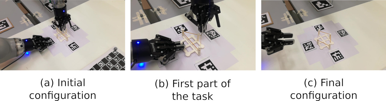
This task consists in manipulating an elastic rubber-band to create a specific shape on a board with sticks (see figure below).

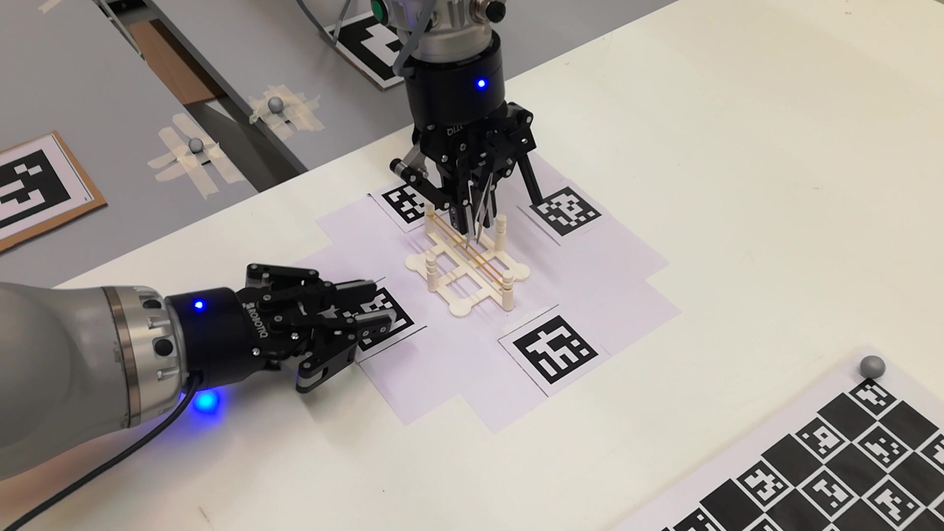
Manipulating the rubber-band requires a control strategy that takes into account the forces generated, which adds one more challenge to the benchmark. The task should be performed by a pair of robotic arms as follows (see also figure below):

One arm holds/supports the tweezers (or similar tool) at its end-effector, while the other arm uses a gripper to stabilize the system. The rubber band is already placed on the board in the initial shape. The arms must manipulate the rubber-band in order to achieve a specific shape on the board.

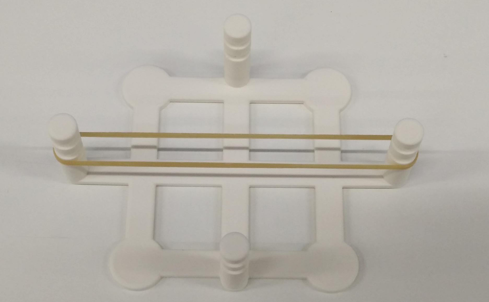
Pieces

For completing the task, one needs the specific board model (see figure below) and a rubber band. Again, to increase reproducibility and ease the 3D printing process, we provide the CAD files of the board along with physical properties.

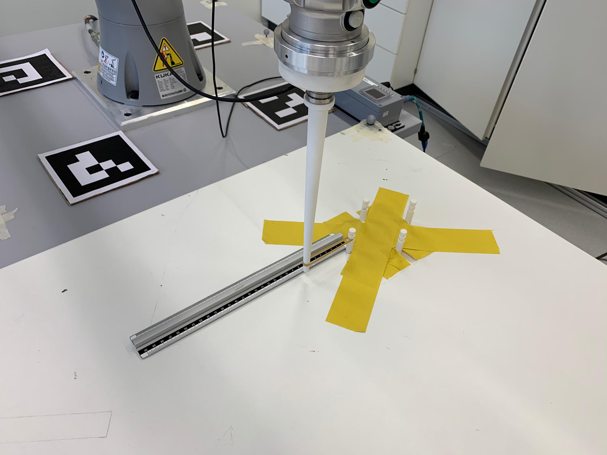
For the rubber band, the users are allowed to use any rubber band with some specific characteristics. To determine the characteristics, the participants need to perform the following: “Measure the force magnitude that the rubber-band produces when stretched at 9cm, 12cm, 14cm and 18cm“. To do-so we propose the following procedure (the participants do not need to follow exactly this procedure): “Use a high-precision manipulator and attach a force-torque sensor at the end-effector (see images below). Fix one tip of the rubber-band to a fixed position and the other tip on the tool of the end-effector. Move the robot to precise locations (a ruler can help to measure them accurately) and calculate the magnitude of the force that is being applied on the force-torque sensor“.

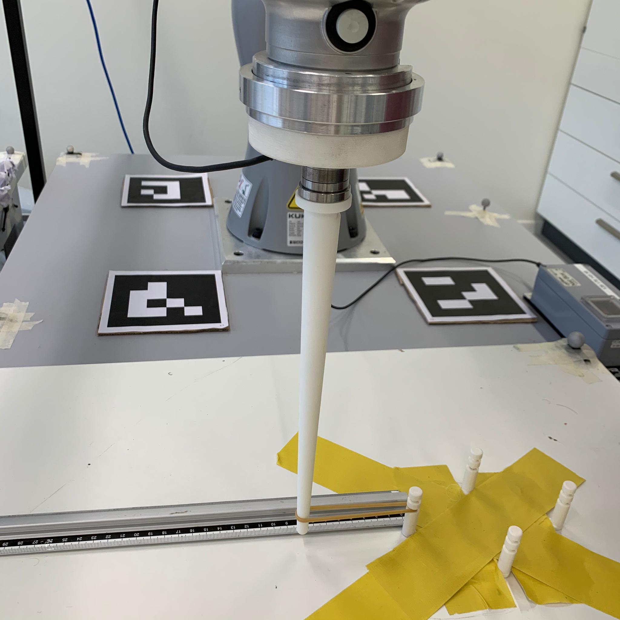
The measured force magnitudes per distance that the utilized rubber-band needs to have (more or less) is as follows:

These values are the average of 3 different measurements of the force magnitude as described above.

CAD Files and Physical properties

You can download the CAD files (STEP files) of the board here. We also include the physical properties of the board in case one wants to use it in simulation. A URDF model will also be available soon (with the physical properties already set).

Tool Constraints

The usage of the tweezers might make the handling of the elastic rubber band easier. However, it may be sufficient to use a standard robotic gripper to replace the tweezer. As in the previous task, we let users decide which option they prefer, and we still impose the same ”pinch” constraint on the end-effector tool. In this case, these constraints apply for both arms since the second arm can also use a robotic gripper to stabilize the system. In fact, the bimanual robotic system can directly manipulate the rubber-band and even not touch the board if so desired.

Submission Categories

The benchmark accepts submissions for approaches that fall in any of the following four categories:

• Adaptive control (AC): in this case, the optimal plan (in kinematic space) to solve the task is assumed to be given and the goal is to find a control algorithm that is able to find the force profiles and adapt to the noisy observations of the computer vision part. No data-driven method is allowed in this category.
• Motion planning (MP) under uncertainty: in this case,the goal is to find a working plan (not given) to solve the task with the ability of handling the uncertainty that comes from the computer vision estimation. No data-driven method is allowed in this category.
• Offline Learning (OFL): in this case, the optimal plan (in kinematic space) to solve the task is assumed to be given or not (this is up to the users to decide; different leaderboards are available per case) and the goal is to find a data-driven algorithm that is able to reliably solve the tasks. In this category, all the learning must be offline, that is, performed only once with the collected real-world samples. Combination of learning methods with motion planning algorithms is allowed.
• Online Learning (ONL): in this case, the goal is to propose a trial-and-error learning algorithm that is able to find a working controller (or policy) that can reliably solve the tasks despite the noisy observations. The algorithm is expected to interact with the system and improve over time. The final optimized controller/policy is evaluated.

More details to be added..

Computer Vision Tracking System

As part of the benchmark we provide a baseline code for inferring the relative transformations between the objects using ChArUco markers and computer vision. We also provide some code to detect the rubber-band assuming white table background (it can easily be adapted to any other constant color). The code is based on OpenCV and python.

The code is available at: https://github.com/epfl-lasa/sahr_benchmark

ChArUco markers setup

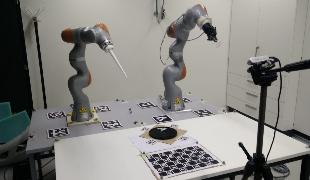
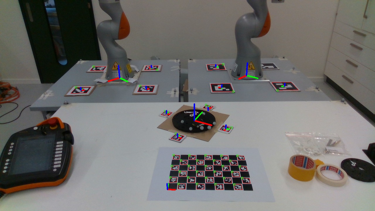
In our setup, we use a single camera to detect all ChArUco markers related to the robots and the watch face (for the first task) or board (for the second task). The camera is placed on the opposite side of the two robot arms. It is placed roughly in the middle so most markers are visible. Four markers from the same ArUco dictionary are placed around each robot arm (although only three are used) and the watch face/board, as shown in the picture above. Each group of four markers must form a perfect square. We use ChArUco chessboard to improve our estimations. Each robot arm, watch face, board, and chessboard is associated with a unique ArUco dictionary. Within an ArUco dictionary, each marker is assigned to an index label. Specifically, in a group of four ArUco markers, the IDs assigned are 0, 1, 2, and 3. OpenCV can detect these markers and output their corresponding IDs. Please note that same IDs are shared across different ArUco dictionaries (i.e., there is a 0-indexed marker in every group of four markers, and same applies for the other markers). This is a nice feature to reduce complexity when we need to address orientation of the markers. In our setup, markers are placed in clockwise order according to their IDs, starting from ID 0. There is no specific orientation for the markers surrounding the watch face/board, since all four markers are visible to the camera. However, for the markers surrounding the robot arms, the marker in the back corner may be occluded by the robot arm. Thus, our computation requires only three markers to be visible for each robot arm. This requires us to enforce a specific orientation of markers: the marker labeled with index 0 is always placed in the bottom left corner. Using three markers per robot and specific orientation, we can construct the coordinate frames correctly. An example of the estimated coordinate frames is shown in the picture below.

Tracking of the rubber-band

Details to be added..

Metrics and Details

Here we provide details about the metrics and how to determine failure cases. We expect potential users of the benchmark to report the performance metrics of their approach per sub-task: (a) watchmaking task with big watch, (b) watchmaking task with small watch, (c) rubber band task. Additionally, the users are expected to report their robotic setup, but also the pipeline of their approach (e.g., whether they used some simulator or not). We define two (2) global metrics that apply to all the submission categories, but also per category metrics.

We set N=5 repetitions, J=3 different initial configurations, and we define the metrics as follows:

Global Metrics

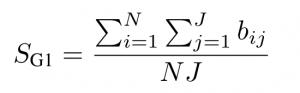
• Success Rate

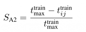
• Average Completion Time

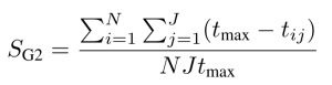
t_ij is the time in seconds required to complete the i-th repetition of the j-th initial configuration. The maximum completion time, t_max, for the task is set to 60 seconds.

Offline Learning Metrics

• Number of offline samples

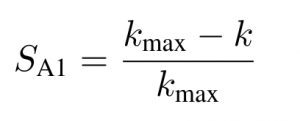
k is the number of offline samples required. The maximum number of offline samples, k_max, is 10000 samples.

Details about what counts as a sample to be added.

• Model Learning Time

The maximum training time is set to 1800 seconds (to be re-visited).

Motion Planning Metrics

• Average Planning Time

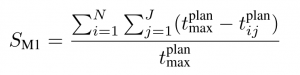
The maximum planning time is set to 1800 seconds.

Online Learning Metrics

• Interaction Time

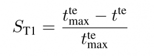
The maximum interaction time is set to 1800 seconds (30 minutes).

Total Score

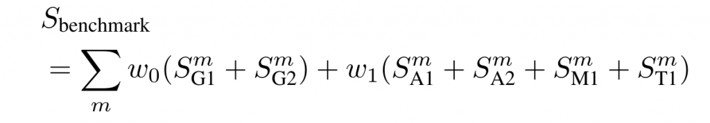
w₀ = 0.25 and w₁ = 0.25/N where N is the number of active scores (apart from G1, G2).

Sub-Metrics

6D pose tracking sub-metric

With this metric, we assess the ability of the robotic system and the controller to achieve 6D poses with millimeter accuracy. We provide a protocol to use the proposed controller to achieve six (6) different end-effector poses, and we measure the distance from the desired pose. The score is defined as follows (the smaller the better):

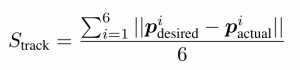
Procedure to be added..

Safe dual-arm end-effector tracking sub-metric

With this metric, we measure the ability of the controller to output collision-free trajectories for the two arms. The robots are given end-effector targets that would lead to a collision using a simple PD-controller (both in end-effector or joint-space), and we measure the following quantities: (a) time in collision, (b) target goal (last point in the path) accuracy. The score is defined as follows (the smaller the better – we iterate over arms i):

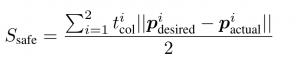
Procedure to determine the two targets to be added..

Force application sub-metric

With this metric, we measure the ability of the controller to apply contact forces in specific directions while maintaining good tracking of the desired end-effector pose. This metric requires a force-torque sensor to be mounted on the end-effector of one of the robots. One of the robots is given a desired end-effector pose and a desired force to apply (the pose should be located within the workspace of the robot and on the table, and the desired force should mostly push towards the table). We let the system run for 10 seconds, and we measure the average error in force (for the whole period) and final end-effector pose error. We do the same procedure for both arms. The score is defined as follows (the smaller the better – we iterate over arms i):

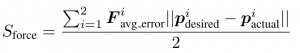
Specific instructions on how to choose the desired force and end-effector pose to be added soon..

Code for Dual-Arm Centralized Control

To define the QP control problem we use our whc C++ library.