Supplementary Material for the EI Newsletter, Special Issue on Smart Image Acquisition and Processing, Vol. 14 (1), January 2004.
David Alleysson & Sabine Süsstrunk
For a copy of the newsletter, go to http://spie.org/web/techgroups/ei/pdfs/ei14-1.pdf.
 |
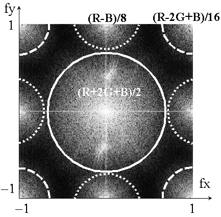 |
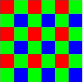
Figure 1: (a) An example of a CFA, the Bayer CFA (b) The Fourier representation of an image acquired with the Bayer CFA.
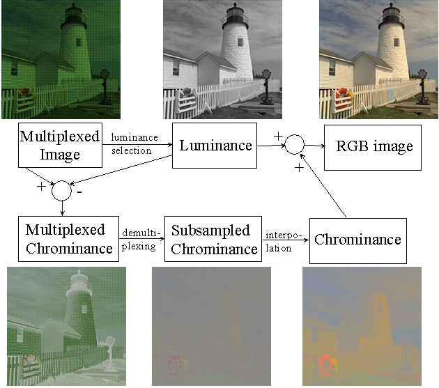
Figure 2: The demosaicing algorithm by frequency selection. A CFA image with a single chromatic sensitivity per spatial location is illustrated at the top-left (the image appears greenish as there are twice more green than red and blue pixels). From this image, we can estimate the luminance (top-middle) with a linear convolution filter that is directly applied to the CFA image. Sub-sampled and modulated chrominance (bottom-left) is estimated by subtracting the luminance from the CFA image. After demodulation (bottom-middle) and interpolation (bottom-right), the chrominance is recovered. By adding chrominance to luminance, a three color per pixel image is formed (top-right).
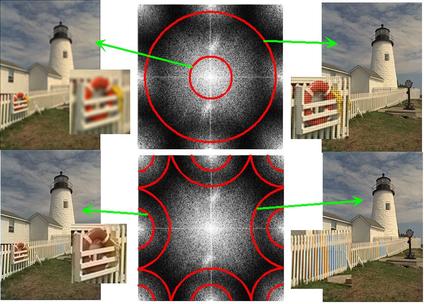
Figure 3: Using a Fourier representation of CFA images, artifacts in demosaicing algorithms can be explicitly demonstrated. If an algorithm estimates luminance with a low-pass filter that is too narrow-band, blurring occurs (top-left). If an algorithm uses a low pass filter whose bandwidth is too broad, we may see grid effects because chrominance information is mixed into the luminance signal (top-right). Similarly for chrominance: if a too narrow high-pass filter is used, water colors or desaturated colors appear that go beyond the boundary of an object. If the high-pass filter is too broad-band, false colors occur because luminance is mixed with the chrominance signal.
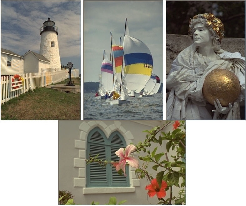
Figure 4: Some image examples using the filter of Figure 5 to estimate luminance.
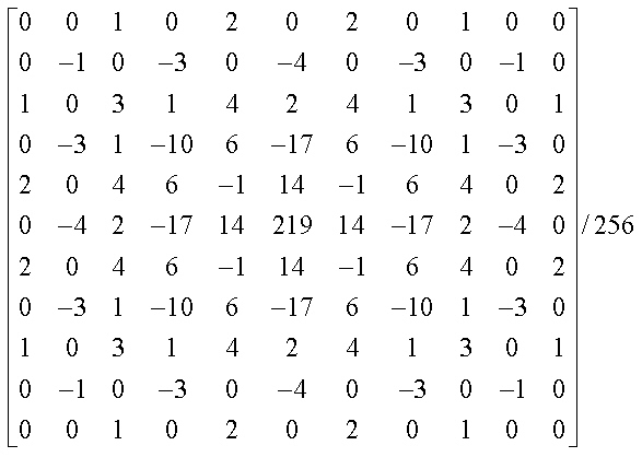
Figure 5: The convolution filter applied to the CFA images to estimate luminance. The results are illustrated in Figure 4.
| Bilinear | Hue Based | Gradient Based |
Alias cancellation | Frequency Selection | |
|---|---|---|---|---|---|
| Lighthouse Time |
25,44 1 |
27.04 1.7 |
31.5 49 |
29.19 13.93 |
34.19 2.71 |
| Sails Time |
28,43 1 |
29.91 1.65 |
34.37 48.21 |
31.07 13.64 |
35.45 2.66 |
| Statue Time |
28,36 1 |
29.66 1.34 |
32.78 48.21 |
31.01 13.63 |
37.7 2.34 |
| Window Time |
27,96 1 |
29.6 1.31 |
31.46 48.87 |
30.91 13.62 |
34.29 2.32 |
Table 1: Comparison of demosaicing by frequency selection to other demosaicing algorithms in terms of color psnr and execution time (demosaicing by bilinear interpolation is taken as one time unit).