Functional Magnetic Resonance Imaging (fMRI) is a technique that allows the visualization of the activity of the brain. It bases on blood flow increases in stimulated areas of the brain. The technique is safe and non-invasive. The simplest experiments consist in switching between periods of rest and period of a basic activity (like looking at a visual stimulus or moving one hand).
The fMRI data is then analysed to identify which areas of the brain have responded to the stimulus by matching the magnetic resonance signal to the stimulus one.
Scientific relevance
Huge neuroimaging datasets are becoming publicly available [1]. One of them is from the Human Connectome Project (HCP) of the NIH. Such datasets should help the scientists to uncover the neural pathways that underlie human brain function.
By the first trimester of 2017, HCP has collected MRI scans from over 1,000 individuals to end up with an impressive collection of brain open data available on the project’s cloud. In particular, high resolution functional MRI (fMRI) scans during resting-state (4 runs per subject, cf. Figure 1) and during tasks (6 runs per subject).

Figure 1: Overview of resting-state fMRI data available in the Human Connectome Project.
The Medical Image Processing Lab (MIP:Lab, EPFL/UNIGE), lead by Professor Dimitri Van De Ville, has built up an extensive expertise in network modeling and dynamical analysis of large-scale human brain activity based on fMRI.
Their data processing pipeline, depicted in Figure 2 below, involves a processing step called Total Activation (TA) that was developed in [2, 3] to retrieve “clean” deconvolved time series reflecting moments of sustained activity in the brain. TA outputs were exploited to explore innovation-driven Co-Activation Patterns (iCAPs) [4] that show spatially and temporally overlapping large-scale networks during brain activity.

Figure 2: Illustration of fMRI processing & analysis pipeline.
Technical aspects
So far the MIP:Lab has run its analysis pipeline on datasets up to 100 runs with limited number of scans per run.
However, being able to process massive data such as the HCP is of major importance for two reasons:
- It is important to further validate that the functional networks established by the iCAPs methodology are robust across large number of subjects.
- New findings can be established when using large datasets such as relationships between network dynamics and neuropsychological traits that are also available for this data, what might also give new insights into brain function and how these networks support cognitive processes.
Results
In the current implementation, the voxels are processed sequentially with the following simplified call stack: MyRegularization → MySpatial → MyTemporal → Temporal_TA. Temporal_TA actually performs a signal denoising with the help of the function filter_boundary, where actually most of the time is spent. filter_boundary is mainly built upon two builtin functions of Matlab: flipud and filter.
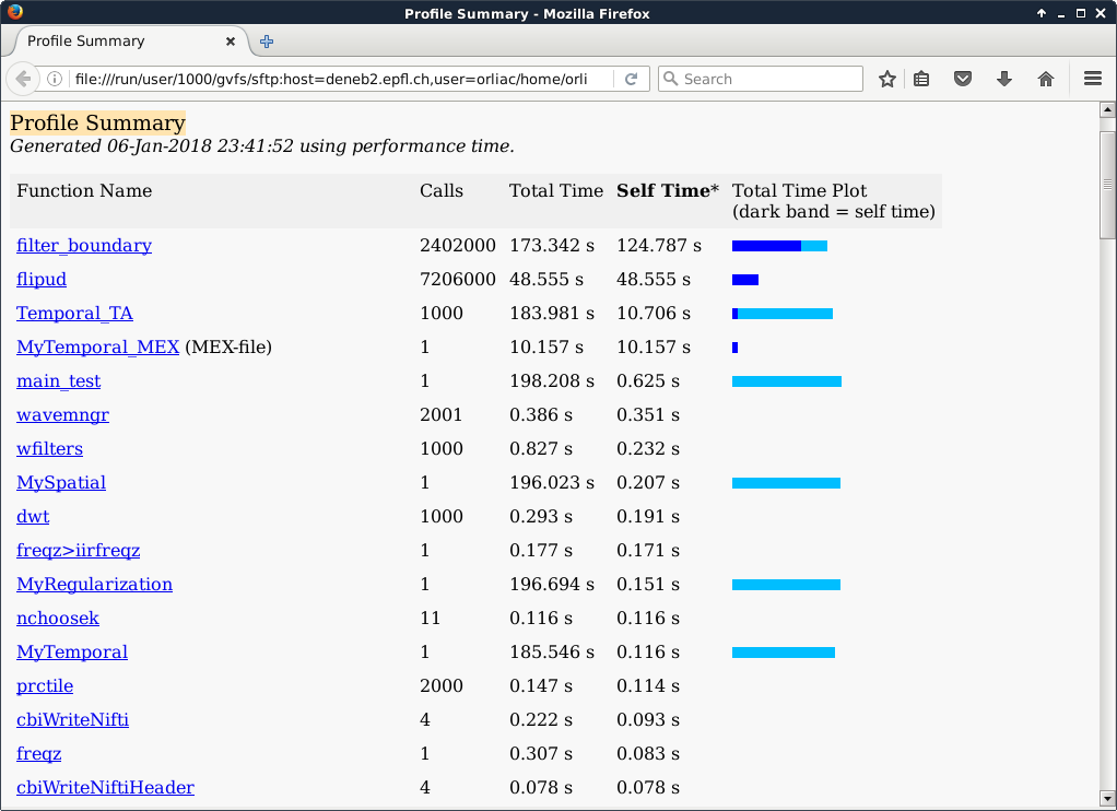
Voxel time courses are looped over in MyTemporal. As exactly the same operations have to be performed for each voxel, it was decided to implement a CUDA kernel to parallelize the time series analysis. The CUDA implementation basically dedicates one thread to one voxel. It was implemented through a Matlab EXecutable (MEX) function (named MyTemporal_MEX) that calls the CUDA kernel.
In the Matlab profiling output presented above, 1000 voxels were processed, hence the 1000 calls to Temporal_TA. MyTemporal took 185.546 s to execute, against 10.157 s for its CUDA couterpart MyTemporal_MEX, i.e. the CUDA implementation performed more than 18 times faster.
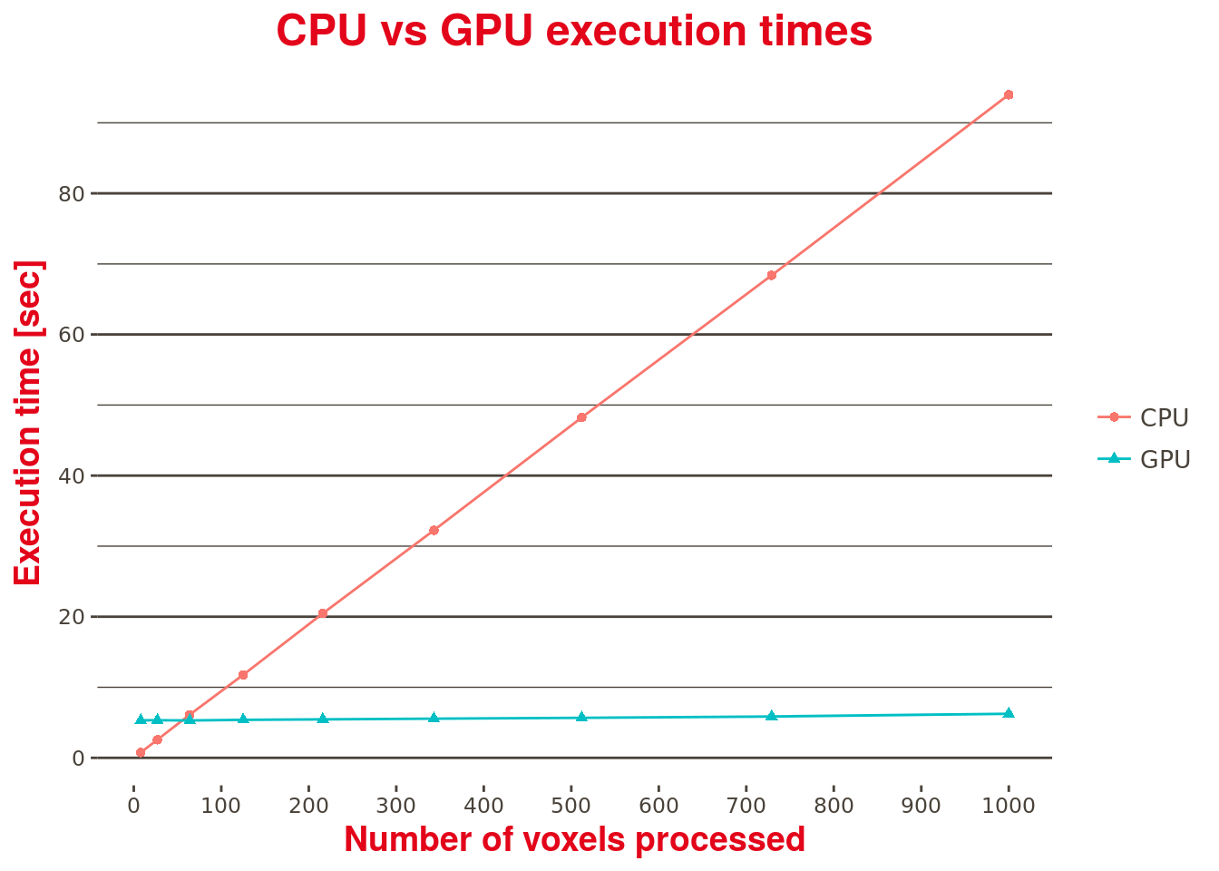
Furthermore, looking at Table 1 below which compares the performances of the CUDA kernel (GPU) over the current (CPU) implementation (this time using timemarks in the code with no Matlab profiler enabled, where both implementations are called) with an increasing number of processed voxels, one can note that the CUDA kernel execution time is almost constant, regardless the number of voxels being processed. A contrario, and as expected, the current and purely sequential CPU based implementation execution time is linearly dependent on the number of voxels processed.
In this test, only 1000 voxels were available. To fully assess the performance improvements brought by the GPU-based implementation, a larger dataset should be considered.
| Number of voxels | CPU | GPU | Execution time improvement factor |
|---|---|---|---|
| 8 | 0.762 | 5.318 | 0.143 |
| 27 | 2.568 | 5.332 | 0.482 |
| 64 | 6.120 | 5.300 | 1.155 |
| 125 | 11.758 | 5.386 | 2.183 |
| 216 | 20.465 | 5.457 | 3.750 |
| 343 | 32.247 | 5.554 | 5.806 |
| 512 | 48.237 | 5.676 | 8.499 |
| 729 | 68.385 | 5.861 | 11.667 |
| 1000 | 93.984 | 6.245 | 15.049 |
Table 1: CPU vs GPU performance comparison.