Fluorescence is the spontaneous re-emission of light by a substance that is exposed to light or another source or electromagnetic radiation, with the wavelength of the re-emitted light being generally greater than that one of the source. A fluorochrome or fluorophore is a substance capable of fluorescence. It can be natural or synthetic but its intensity profiles of excitation and emission have to be accurately known to be useable in microscopy. In fluorescence microscopy, the available fluorochromes allow to stain specific structures to be observed or serve as indicators or probes of certain conditions of the observed environment.
One drawback of the fluorescence microscopy is its low spatial resolution due to light diffraction. [Huang et al., 2009] indicate resolutions of 200-300 nm and 500-700 in the lateral and radial directions respectively. To overcome this limitation, the so-called super-resolution fluorescence microscopy techniques have been developed (see [Huang et al., 2009] for a review). For the best techniques, the spatial resolution can reach 10 nm in optimal conditions, among which the STORM (STochastic Optical Reconstruction Microscopy) and PALM (PhotoActivated Localization Microscopy).
Scientific relevance
The superior resolutions of STORM and PALM have proven to be invaluable to molecular biologists as they have, for example, determined the structure of the nuclear pore complex, actin cortical rings, the bacterial division machinery, and the structure of telomeres.
Despite their success, STORM and PALM are relatively low throughput techniques due to their long acquisition times, which limits their use to relatively orderly macromolecular structures in a small number of cells. Inherently disordered structures, such as the DNA polymer, are difficult to study in their native cellular environment because the severe limit on the size of the datasets prevents scientists from adequately sampling all of the possible conformations and the resulting cellular phenotypes. On the other hand, super-resolution fluorescence techniques are arguably more suited to this task than electron microscopy (EM) because the specificity of EM is not sufficient to discern the numerous protein species that associate to a disordered macromolecular complex.
The LEB, the Laboratory of Experimental Biophysics of EPFL, currently develops high-throughput techniques that leverage advances in automation and machine learning to take advantage of the high resolution and specificities of super-resolution fluorescence microscopy while simultaneously overcoming the selection bias and poor sampling of their original implementations. Combined with computational modeling approaches, the LEB is applying high-throughput STORM to build a spatial map of proteins in the centriole and to visualize the structure-function relationship of the DNA polymer.
Technical aspects
The key principle of STORM/PALM is to allow only one fluorescent molecule to emit light within a diffraction-limited area (approximately 1 square micrometer) at a time. The processus of identifying and extracting these areas, or spots, in raw images is referred to as segmentation. If a single fluorescent spot is known to contain only one emitting fluorophore, then that fluorophore’s position may be determined with nanometer accuracy by fitting the image to a two-dimensional Gaussian and taking the center of the fit to be the molecule’s position. This step is referred to as localization hereinafter, and can be performed on each spot, fully independently from all other spots.
Localization is computationally intensive since it is performed on tens of thousands of images and millions of spots per acquisition. Numerous algorithms and software libraries have been developed to handle this task. They rely on fitting techniques such as weighted least-squares, maximum likelihood estimates of the spot centers, and phase retrieval.
Despite their algorithmic differences, nearly all current libraries for STORM/PALM are designed to work on single CPU cores because the historically low throughput of the techniques have not produced enough data to justify the development of faster implementations. The new highthroughput approaches, however, are generating terabytes of image data per day, surpassing the old approaches by more than an order of magnitude. Processing datasets of this size takes pohibitively long amounts of time, even when using GPU-based libraries such as the one used at LEB: one day of imaging currently requires 12 – 18 hours of post-processing on a single workstation.
The situation will get even more dramatic as new methods are being developped at LEB that should soon increase acquisition rates tenfold, which would lead, with the current situation, to post-processing times of several days.
Fortunately, the overall processing scheme is embarrassingly parallel. Each raw image is independent of all the other images, and the location of the individual fluorescent spots in an image is completely independent of all the other spots. This means that both the spot finding and the localization steps may be performed in parallel with an increase in speed that should scale linearly with the number of cores available.
Data workflow
The current dataflow at LEB is presented in Fig. 1. The microscope generates one image every 10 ms. Each image is 500 x 500 up to 2’000 x 2’000 pixels. Each pixel is encoded with 16 bits. It means that, at maximum, the microscope produces 0.8 GB/s of data, what would correspond to 69.12 TB/day if it were operated continuously.
The segmentation extracts small square portions of size 7 x 7 up to 21 x 21 pixels of the raw images containing fluorescence “spots”. Those extracted spots represents roughly 10 % of the original image size.
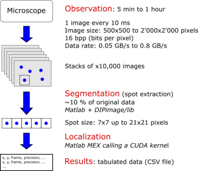
Figure 1: Current dataflow at LEB.
Work performed
CUDA kernel improvement and optimizations
The core of kernel was kept but the following improvements were brought:
- Elimination of expansive or useless mathematical operations
- Simplification of expressions
- Dynamic shared memory allocation (instead of allocating by default the maximum potentially needed for the 21 x 21 pixels subregions)
- Optimization for the processing of 7 x 7 pixels subregions: a single warp (32 threads) is used to process the 49 pixels, rather than using blocks of 49 threads.
New routine for the image segmentation
So far, only an executable for Windows platforms was available to carry out the image segmentation (cMakeSubregions.mexa64, authored to Keith Lidke). Since it was not possible to obtain the source code, it was decided to reimplement it. What the function does is rather straightforward: it simply extracts small square portions in the raw image around given positions. If the image portions to extract fall outside the image, the center are simply shifted to completely be on the image. The new routine, cMakeSubregions2.c, is provided as a C MEX file (i.e. fully portable).
An improvement was brought thought to the new routine: it accepts both 2D and 3D input data, as opposed to the original version that was only acception 3D data. It means that invariant input data such as 2D variance or gain maps of the used camera chip do no longer need to be replicated as many times as the number of spots to be treated to extract corresponding subregions.
Memory blowup removal
The implementation of the new segmentation routine described in the above paragraph allowed to solve a memory “blow up” that was due to the useless replication of the same information (2D variance and gain maps of the used camera chip) to perform element-wise (or pixel-wise) operations on each subregions. To that end, the operations involving explicitly replicated matrices using the repmat function of Matlab calls where replaced by Matlab bsxfun calls, where implicit replication is carried out if necessary.
Results
In this section we present a comparison of the performance between the original version of the code and new ones. To that end, we use a reference dataset, based on simulated data, consisting of a stack of 15’000 images, each image being of size 68 x 68 pixels, and containing overall of total of 176’000 spots/subregions. Each spot has a size of 7×7 pixels. This reference dataset is referred to as DSREF hereinafter.
The two improvements detailed above (new routine for the image segmentation and solving the memory blowup) are used in all solutions presented here. All solutions were computed on a GPU node of the deneb cluster managed by SCITAS. The GPU devices are Tesla K40m from Nvidia.
The comparison, summarized in Table 1, focuses on the CUDA kernel execution time and the following solutions are compared:
- REF: the reference solution, generated with the original code, static shared memory allocation, single GPU.
- SC1: solution with optimized code, dynamic shared memory allocation, single GPU.
- SC2: solution with optimized code but using a single wrap (32 threads) for each spot (even though the spot size > warp size). For now this solution is only available when dealing with 7×7 subregions. This solution uses static shared memory allocation and a single GPU.
- SC2_opt: same as SC2, but with the CUDA kernel compiled with some optimization with respect to the maximum number of registers per block (–maxrregcount=48 in this case).
Table 1: CUDA kernel execution times
| Solution | Grid size | Block size | Max. registers per thread | Registers per thread | Shared mem. per block [KiB] | Occupancy achieved / theoretic [%] | Kernel execution time [ms] | Improvement factor |
|---|---|---|---|---|---|---|---|---|
| REF | 176’409, 1, 1 | 49, 1, 1 | – | 86 | 5.531 | 24.8 / 25.0 | 3’202 | 1.00 |
| SC1 | 176’409, 1, 1 | 49, 1, 1 | – | 50 | 0.948 | 49.6 / 50.0 | 1’258 | 2.54 |
| SC2 | 88’205, 1, 1 | 64, 1, 1 | – | 74 | 1.859 | 37.4 / 37.5 | 865 | 3.70 |
| SC2_opt | 88’205, 1, 1 | 64, 1, 1 | 48 | 48 | 1.859 | 49.7 / 50.0 | 646 | 4.96 |
Bottom line: with the optimized code compiled with specific options, we managed to reduce the kernel processing time by a factor of 5!
Note: the computations are carried out using single precision. Changes brought in the kernel brought slight differences in the results but were acknowledged as very acceptable by the LEB.
As shown in Fig. 2 below, with this reduced dataset, there is a significant time spent on the first CUDA stream creation “cudaStreamCreate”, that lasts for more than 300 ms, roughly half the actual kernel processing time. In fact, this is the first call to CUDA, and therefore contains an implicit call to the CUDA context creation, which is imcompressible in time.
To hide the induced latency, the throughput should be maximized when the kernel is deployed in production. We recall here that the present assessment was carried out on a reduced synthetic dataset. Real datasets contains millions of spots, here we used less than 200’000.
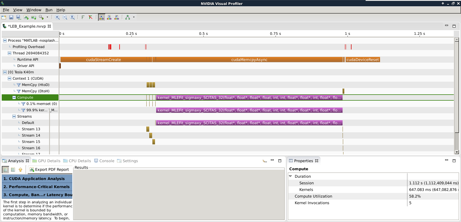
Figure 2: Screenshot of the Nvidia Visual Profiler output for the best performing kernel.
Proposed workflow
The new workflow below was proposed. After discussion with the LEB, it appeared more suitable to continue carrying out the image segmentation on the actual acquisition station, as the resources allow it and it avoids transferring the full images for processing. Only the subregions/spots are sent to a data node.
The data node, upon reception of new data, will trigger the processing (localization) on one or several GPU compute nodes of the cluster. On successful completion of the localization, the results are transferred to the scientific storage. After completion of a cycle, the scientific storage will hold all the data: raw data, subregions, and the results.
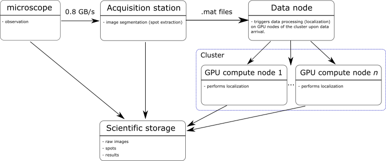
The obvious advantage of the proposed new workflow is the ability to scale to compute power on demand and process data in real-time.