As of November 2015, we have a working demo of Commelec.
The demo setup consists of:
Commelec Grid Agent
a fully-controllable battery
an uncontrollable PV system
a fully-controllable load that mimics eight 1kW electrical on-off heaters
a microgrid (about 1 km of cables)
We have defined two demo-experiments:
1. Tracking a sinusoidal power request at the slack bus (the point of common connection to the upper-level grid)
2. Providing a primary frequency-control service to the main grid
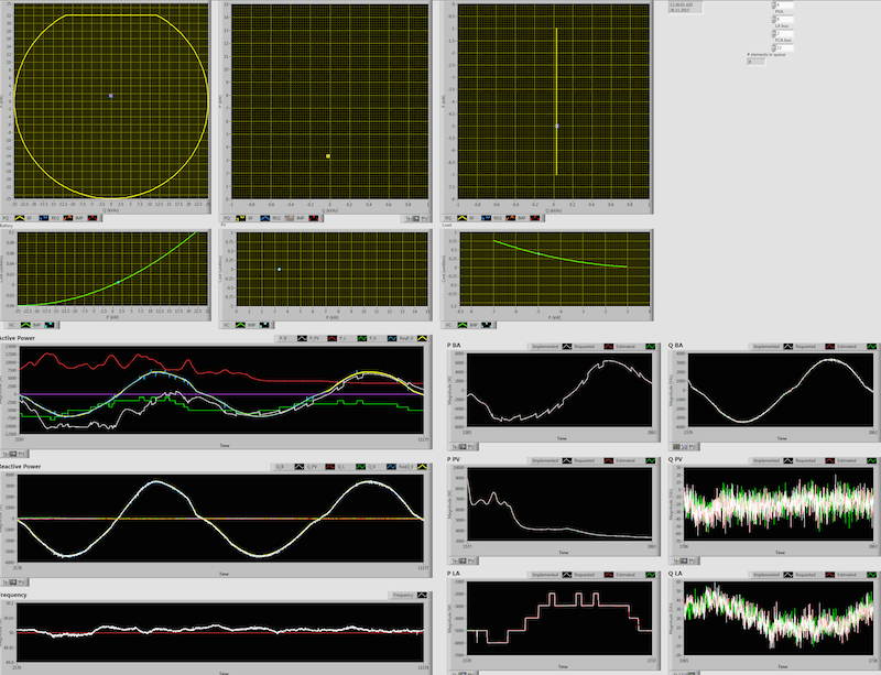
Below, you see a screenshot from the SCADA. The window titled “Active Power” shows the sinusoidal target (yellow, mostly covered by the cyan curve), and the measured power at the slack bus (cyan), the power consumed by the heaters (green), and the battery (white). Note how the battery and the heating system use their flexibility to contribute to following the sinusoidal target.
In the upper left figure, you see the PQ profile of the battery and the currently implemented setpoint. Below that, in green, the cost function is displayed (evaluated along the real-power axis).
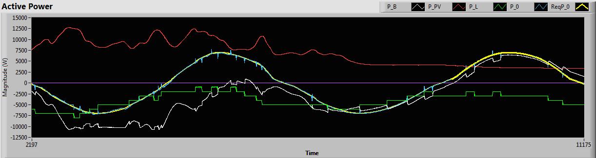
A zoomed version of the graph that shows the real-power injection/consumption of the resources in the demo setup.
In particular, note how the PV injection varies (the red graph), and how the battery (white graph) as well as the flexible-heating system (green time series) automatically and jointly compensate for these fluctuations, so that the power consumption at the connection point (to the medium-voltage grid) follows the yellow target time series.
Below, we show a sample of the console output of the grid agent:
----=== COMMELEC cycle ===----


Simulation Mode Enabled: Grid's state and bus power injections are computed from the
                  ImplementedSetpoint-field from the follower advertisements.
Slack Bus Power, requested (a sinusoid): P = 2286.83 Q = 1107.56
Slack Bus Power, computed via load-flow: P = 2249.79 Q = 1123.66
Computing Setpoints...

Follower: battery (Agent Id: 12, Bus Id: 4)
    Cost Gradient:    P = 48.9119, Q = 0
    Voltage Gradient: P = 0.0130435, Q = 0.522389
    Current Gradient: P = 0, Q = 0
    Request gradient: P = -42.037, Q = 0.0220935
    Implemented Setpoint (as reported by RA) P: 5569.92, Q: 1047.57
    Estimated Bus-Power Injection P: 5569.92 [W], Q: 1047.57 [VAR]
    Candidate Power Setpoint (before projection onto the safety set):  P: 5563.03 [W], Q: 1047.54 [VAR]

Follower: uncontr-gen (Agent Id: 15, Bus Id: 8)
    Cost Gradient:    P = 0, Q = 0
    Voltage Gradient: P = 0.0219793, Q = 0.739276
    Current Gradient: P = 0, Q = 0
    Request gradient: P = -42.0888, Q = 0.0133819
    Implemented Setpoint (as reported by RA) P: 668.589, Q: -11.2911
    Estimated Bus-Power Injection P: 668.589 [W], Q: -11.2911 [VAR]
    Candidate Power Setpoint (before projection onto the safety set):  P: 710.656 [W], Q: -11.3118 [VAR]

Follower: loadagent (Agent Id: 18, Bus Id: 2)
    Cost Gradient:    P = -1.24093e-06, Q = 0
    Voltage Gradient: P = -0.00370531, Q = 0.258017
    Current Gradient: P = 0, Q = 0
    Request gradient: P = -42.345, Q = 0.0108913
    Implemented Setpoint (as reported by RA) P: -3970.97, Q: 26.7827
    Estimated Bus-Power Injection P: -3970.97 [W], Q: 26.7827 [VAR]
    Candidate Power Setpoint (before projection onto the safety set):  P: -3928.62 [W], Q: 26.7692 [VAR]

Setpoint computation done (Total time: 0.823287 ms.)
Computed setpoints for the upcoming requests (after the projection step):
battery -----------------> P: 5563.03, Q: 1047.54
uncontr-gen -------------> P: 660.801, Q: -11.2911
loadagent ---------------> P: -4000, Q: 26.7827
Cycle Time: 191 ms.
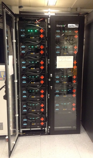
The battery stack.
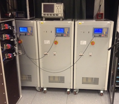
The controllable loads.